Galerkin neural networks for approximating PDEs
1. Introduction
Neural networks have seen much success in computer vision over the last decade. Only more recently has there been an increase in interest in using them for tasks that have traditionally been in the purview of computational scientists and engineers. The one task I’d like to discuss today is approximating solutions of PDEs. To my knowledge, the first use of neural nets for this task was by Dissanayake and Phan-Thien in [1]. They proposed learning solutions by minimizing the interior and boundary residuals associated with the PDE measured in the \(L^{2}\) norm.
As computational power and optimization techniques have improved, neural networks have only grown more in popularity. For solving the forward PDE problem, most works in the literature today are similar to the approach in [1]. It is also worth noting that neural networks offer clear advantages for high-dimensional PDEs and problems for which one would like to incorporate measured data alongside a physics-based model, see for instance physics-informed neural networks.
However, in practice there are a number of issues that arise when using neural networks to approximate PDEs. The most glaring is that while neural networks are universal approximators, their associated objective functions are highly nonconvex and one often observes that the approximation error stagnates after a certain point irrespective of how many layers or neurons are added to the network. This is in sharp contrast with traditional methods such as finite elements which have theoretical guarantees on the error that are realized in practice.
Our goal when developing Galerkin Neural Networks was to have an approach that allows for rigorous control of the approximation error. Leveraging techniques from functional analysis, we train a sequence of shallow networks which learn Riesz representers of weak residuals of the PDE. These Riesz representers form a finite-dimensional subspace from which to approximate the PDE. The result is a method that I believe stands apart quite distinctly from other approaches in the literature. The full analysis and results may be found in my paper [2] (co-authored with my advisor Mark Ainsworth), but this post serves as an accessible introduction with accompanying code.
2. Feedforward Neural Networks
Mathematically, a feedforward neural network is best described as a linear combination of parameterized nonlinear functions. To be precise:
Definition 1. Given an input \(x \in \mathbb{R}^{d}\), the feedforward neural network with \(\ell\) hidden layers and widths \(n_{0}, \dots, n_{\ell}\) is described by the sequence of linear transformations
\[\begin{align} T_{i}(x) = \begin{cases} x\cdot W^{(i)} + b^{(i)}, &i=1,\dots,\ell-1\\ x\cdot c, &i=\ell \end{cases} \notag \end{align}\]and the function \(u_{NN} : \mathbb{R}^{d} \to \mathbb{R}\) given by
\[\begin{align} u_{NN}(x;\theta) := T_{\ell} \circ (\sigma \circ T_{\ell-1} \circ \dots \sigma \circ T_{i} \circ \dots \sigma \circ T_{1})(x), \end{align}\]where \(W^{(i)} \in \mathbb{R}^{n_{i-1}\times n_{i}}\), \(b^{(i)} \in \mathbb{R}^{1\times n_{i}}\), \(c \in \mathbb{R}^{n_{\ell}}\), and \(\sigma : \mathbb{R} \to \mathbb{R}\).
In the standard nomenclature, \(W^{(i)}\) and \(b^{(i)}\) are the weights and biases, respectively, of the \(\ell\)th hidden layer; \(c\) are the linear or activation coefficients; and \(\sigma\) is the activation function. Often \(\theta\) is used to denote all of the network parameters \((W^{(i)}, b^{(i)})\) and \(c\).
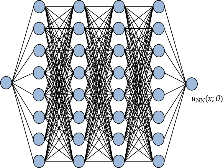
As an example, for \(\ell=1\) we can write \(u_{NN}\) as
\[u_{NN}(x;\theta) = \sum_{i=1}^{n} c_{i}\sigma(x\cdot W^{(1)}_{i} + b^{(1)}_{i})\]which allows us to more easily see that this is really just a linear combination of nonlinear functions. Some common choices of \(\sigma\) are the ReLU function \(t \mapsto \max\{0,t\}\), the hyperbolic tangent function, and the sigmoid function \(t \mapsto 1/(1+\exp(-t))\). For our work, we only use the hyperbolic tangent function.
The goal of a neural network is to determine, or “learn”, the parameters \(\theta\) such that \(u_{NN}(\cdot;\theta)\) is a good approximation to some given target function \(f\). For instance, suppose we simply want to fit a feedforward neural network to \(f\). A common approach is to compute
\[\begin{align} \theta^{*} = \text{arg min}_{\theta} ||f-u_{NN}(\cdot;\theta)||_{L^{2}}^{2} \label{eq:objective fn} \end{align}\]in order to learn the optimal parameters \(\theta^{*}\). A problem such as \eqref{eq:objective fn} is typically approximated using a first-order method, such as stochastic gradient descent, or a second-order method, such as BFGS. We’ll discuss some particular optimization methods for training neural networks later in this post.
II. Approximation of PDEs via Neural Networks
In [1], the authors consider a PDE of the form
\[\begin{align} \begin{cases} \mathcal{L}[u] = f, &\text{in}\;\Omega\\ \mathcal{B}[u] = g, &\text{on}\;\partial\Omega, \end{cases} \notag \end{align}\]where \(\mathcal{L}\) and \(\mathcal{B}\) are differential operators. They propose the minimization problem
\[\begin{align} \min_{\theta} ||\mathcal{L}[u_{NN}(\cdot;\theta)] - f||_{L^{2}(\Omega)}^{2} + ||\mathcal{B}[u_{NN}(\cdot;\theta)] - g||_{L^{2}(\partial\Omega)}^{2} \label{eq:dissanayake objective} \end{align}\]in which one seeks to minimize both the interior and boundary residuals evaluated at a discrete set of points in the domain. A similar approach is followed in physics-informed neural networks.
There are a few things worth noting before we continue.
-
The optimization problem \eqref{eq:dissanayake objective} only makes sense if \(f \in L^{2}(\Omega)\) and \(g \in L^{2}(\partial\Omega)\). There are many instances where we might have \(f \in H^{-1}(\Omega)\), for example \(f = \delta_{0}\) where \(\delta_{0}\) is the Dirac-Delta distribution. In this case, a pointwise interpretation of the residuals does not make sense.
-
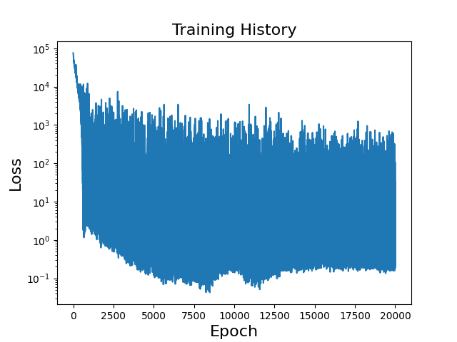
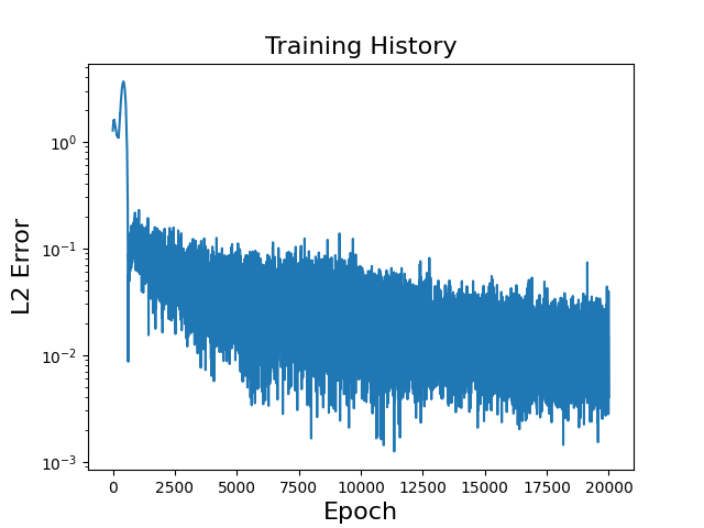
Despite neural networks having excellent approximation power in theory, their approximation error often stagnates after a certain point and increasing network width and/or depth does not typically solve this issue. This stagnation can be due to stalling in local minima, which has been written about in the context of function approximation here, but in general, one can’t expect to specify a target approximation error – say, maybe we want our \(L^{2}\) error to satisfy \(\|f - u_{NN}(\cdot;\theta)\|_{L^{2}} < \mathcal{O}(10^{-4})\) – and expect to to be able to achieve this. This is in contrast to methods such as finite elements where, provided a stable discretization is chosen, machine precision error can be reached even if getting there is computationally infeasible.
Example 1. To demonstrate the second point above, we attempt to learn the solution to the differential equation \(-u''(x) = f(x)\) with homogeneous Dirichlet boundary condition (i.e. \(u(0) = u(1) = 0\)). The true solution is taken to be
\[u(x) = \sin(2\pi x) + \sin(4\pi x) + \sin(6\pi x)\]and \(f\) is chosen to satisfy this true solution. The loss history over each epoch is provided in Figure 2 alongside a table of parameters for the implementation.
\(\small \begin{array}{c|c|c|c|c|c|c|c} \hline \textbf{Parameter} & \text{depth} & \text{width} & \text{activation} & \text{optimizer} & \text{learn rate} & \text{training set} & \text{batch size} \\ \hline \textbf{Value} & \text{2} & \text{150, 150} & \tanh & \text{Adam} & 10^{-5} & \text{20000} & \text{50} \\ \hline \end{array}\)
We can repeat this example with deeper or wider networks and find that while initially, such architectures might yield an increase in accuracy, they eventually won’t decrease the approximation error further. In fact, haphazardly using very deep networks can yield worse results due to difficulty in training.
Before I talk about Galerkin neural networks and how they attempt to skirt around this issue, we’ll need to (briefly) cover variational formulations and weak solutions of PDEs.
3. Overview of Variational Formulations for PDEs
We’ll start out with a motivating example here. Let \(X\) be a general Hilbert space (we’ll be more concrete in a second, but \(X\) is just a space of functions with some restrictions on their behavior). Let’s multiply the equation from Example 1 (\(-u''(x) = f(x)\)) by a function \(v \in X\) and integrate both sides over the interval \((0,1)\):
\[-\int_{0}^{1} u''(x)v(x)\;dx = \int_{0}^{1} f(x)v(x)\;dx.\]The integral on the left-hand side can be integrated by parts to obtain
\[\begin{align} \int_{0}^{1} u'(x)v'(x)\;dx - u'(1)v(1) + u'(0)v(0) = \int_{0}^{1} f(x)v(x)\;dx.\label{eq:weak form ex1} \end{align}\]The Hilbert space \(X\) is typically chosen according to the highest order of derivatives appearing in \eqref{eq:weak form ex1} as well as the boundary conditions for the equation. In this case, we’ll work with the Sobolev space \(H^{1}_{0}\):
\[H^{1}_{0}(\Omega) := \left\{ v \;:\; \int_{\Omega} |D^{\alpha}v|^{2}\;dx < \infty, \;|\alpha| \leqslant 1, \;v|_{\partial\Omega} = 0\right\}.\]The space \(H^{1}_{0}\) consists of function whose derivatives up to first-order are square integrable and whose value on the boundary of the domain is zero. We note that if \(v \in H^{1}_{0}\), then the boundary terms in \eqref{eq:weak form ex1} will vanish and we’re left with
\[\int_{0}^{1} u'(x)v'(x)\;dx = \int_{0}^{1} f(x)v(x)\;dx.\]The \(H^{1}_{0}\) variational or weak formulation of Example 1 is to seek a solution \(u \in H^{1}_{0}(0,1)\) such that \(\begin{align} \int_{0}^{1} u'(x)v'(x)\;dx = \int_{0}^{1} f(x)v(x)\;dx \;\;\;\forall v \in H^{1}_{0}(0,1).\label{eq:poisson1d weak} \end{align}\)
If you haven’t taken a course on PDEs before \eqref{eq:poisson1d weak} will probably be quite new to you, so I want to point out a few key observations.
-
Any \(u\) which satisfies \(-u''(x) = f(x)\) for \(x \in (0,1)\) and \(u(0)=u(1)=0\) will automatically satisfy \eqref{eq:poisson1d weak}. This is clear by following the derivation steps above. So what does this mean? If the data \(f\) is smooth enough, it means that the solution of the original equation and the solution of \eqref{eq:poisson1d weak} coincide.
-
\eqref{eq:poisson1d weak} only involves first derivatives of \(u\) and \(v\) while our original equation involved second derivatives. Since requiring the existence of second derivatives is a stronger condition, we can surmise that solutions of \eqref{eq:poisson1d weak} are “weaker” than solutions of the original equation, hence where the term weak solution comes from. For most cases, when the data \(f\) is smooth enough (and in two dimensions and higher, when the domain is regular enough), this weakening of the required smoothness of the solutions is irrelevant. However, there will be genuine cases that occur in practice, especially in solid and fluid mechanics, where solutions contain discontinuities, boundary layers, and sharp gradients which reduce regularity for which weak formulations such as \eqref{eq:poisson1d weak} are necessary. We’ll touch more on this later.
-
Rather than requiring an equation to be satisfied for every value of \(x\), \eqref{eq:poisson1d weak} only considers averaged quantities. That is, as long as the integrals in \eqref{eq:poisson1d weak} are finite, its solution is well-defined. This is in contrast to the original equation (whose solutions we’ll refer to as classic solutions) which requires \(u''(x)\) to be defined for all \(x\) in the domain in order for a solution to make sense.
Even when it’s not strictly necessary to use a weak/variational formulation like \eqref{eq:poisson1d weak}, numerical methods such as finite elements work with the variational formulation since its approximation is usually equivalent to solving a sparse linear system of equations. As well, there are a number of mathematical tools that allow for proving nice error estimates when working with the weak formulation.
I. Approximating Weak Solutions
With all that out of the way, how do we actually solve a variational equation like \eqref{eq:poisson1d weak}? To generalize things a bit more nicely, let’s consider an abstract variational problem on a Hilbert space \(X\):
\[\begin{align} u \in X \;:\; a(u,v) = L(v) \;\;\;\forall v \in X.\label{eq:variational} \end{align}\]Here, \(a : X \times X \to \mathbb{R}\) is a bilinear operator on \(X\) and \(L : X \to \mathbb{R}\) is a linear operator on \(X\). In the previous example, we would have \(a(u,v) := \int_{0}^{1} u'(x)v'(x)\;dx\) and \(L(v) := \int_{0}^{1} f(x)v(x)\;dx\). Typically, \eqref{eq:variational} can’t be solved exactly and we’ll have to seek an approximate solution.
Definition (Galerkin method). Given a finite-dimensional subspace \(X_{h} \subset X\), the Galerkin method seeks an approximate solution to \eqref{eq:variational} which is an orthogonal projection (with respect to the bilinear operator \(a(\cdot,\cdot)\)) of the true solution \(u\) onto \(X_{h}\). This is equivalent to seeking a solution \(u_{h} \in X_{h}\) such that
\[\begin{align} a(u_{h},v) = L(v) \;\;\;\forall v \in X_{h}.\label{eq:galerkin} \end{align}\]What does the Galerkin method actually entail in practice? If \(X_{h}\) is a finite-dimensional space of \(X\), then it is spanned by a (finite) set of basis functions which we’ll denote by \(\{\varphi_{i}\}_{i=1}^{n}\). In other words, we can write \(X_{h} = \text{span}\{\varphi_{i}\}_{i=1}^{n}\). This means we can write \(u_{h}\) as \(u_{h}(x) = \sum_{j=1}^{n} c_{j}\varphi_{j}(x)\) for some coefficients \(c_{j}\), i.e. \(u_{h}\) is simply a linear combination of the basis functions of \(X_{h}\) and solving \eqref{eq:galerkin} is equivalent to finding the linear coefficients \(c_{j}\) so that \(u_{h}\) satisfies \eqref{eq:galerkin}.
In order for \(u_{h}\) to solve \eqref{eq:galerkin}, we must have \(a(u_{h},v) = L(v)\) for each \(v \in X_{h}\). Since there are finitely many basis functions in \(X_{h}\), this is then equivalent to the system of equations
\[\begin{align} a(\sum_{j=1}^{n} c_{j}\varphi_{j}, \varphi_{1}) &= L(\varphi_{1})\notag\\ a(\sum_{j=1}^{n} c_{j}\varphi_{j}, \varphi_{2}) &= L(\varphi_{2})\notag\\ &\vdots\notag\\ a(\sum_{j=1}^{n} c_{j}\varphi_{j}, \varphi_{n}) &= L(\varphi_{n}).\label{eq:system1} \end{align}\]To solve for \(c\), we note that \(a\) is linear in the first argument so \eqref{eq:system1} can be written as the linear system
\[\begin{align} \begin{bmatrix} a(\varphi_{1}, \varphi_{1}) & a(\varphi_{1}, \varphi_{2}) & \cdots & a(\varphi_{1}, \varphi_{n})\\ a(\varphi_{2}, \varphi_{1}) & a(\varphi_{2}, \varphi_{2}) & \cdots & a(\varphi_{2}, \varphi_{n})\\ \vdots & \vdots & \ddots & \vdots\\ a(\varphi_{n}, \varphi_{1}) & a(\varphi_{n}, \varphi_{2}) & \cdots & a(\varphi_{n}, \varphi_{n}) \end{bmatrix} \begin{bmatrix} c_{1}\\ c_{2}\\ \vdots\\ c_{n} \end{bmatrix} = \begin{bmatrix} L(\varphi_{1})\\ L(\varphi_{2})\\ \vdots\\ L(\varphi_{n}) \end{bmatrix}.\label{eq:discrete} \end{align}\]Notably, the Galerkin method yields a solution which is the “best approximation” to \(u\) from the space \(X_{h}\), a fact which was proved by Jean Céa in his 1964 dissertation.
Theorem (Céa’s Lemma). Let \(X\) be a Hilbert space with norm \(||\cdot||_{X}\). Let \(a : X \times X \to \mathbb{R}\) ve a bilinear operator which is both continuous and coercive in \(X\), i.e.
-
There is a constant \(M > 0\) such that \(a(u,v) \leqslant M\|u\|_{X}\|v\|_{X}\) for all \(u,v \in X\) (continuity),
-
There is a constant \(\alpha > 0\) such that \(\alpha \|v\|_{X}^{2} \leqslant a(v,v)\) for all \(v \in X\) (coercivity).
Then \(u_{h}\) defined by \eqref{eq:galerkin} satisfies the estimate
\[\begin{align} \|u-u_{h}\|_{X} \leqslant \frac{M}{\alpha} \inf_{v \in X_{h}} \|u-v\|_{X} \label{eq:cea}. \end{align}\]The continuity and coercivity conditions relate to the well-posedness of \eqref{eq:variational}. They are sufficient conditions for \eqref{eq:variational} to have a unique solution. Céa’s Lemma is useful because \eqref{cea} allows us to leverage approximation properties of the space \(X_{h}\) to derive error estimates for the PDE approximation \(u_{h}\). What exactly do we mean by this? Let’s demonstrate with an example.
In finite element methods, one takes \(X_{h}\) to be the space of piecewise continuous polynomial functions. In one dimension, the basis for piecewise linears are the hat functions. The approximation error of any continuous function by such functions may be quantified by the size of the support of each hat function (i.e. the so-called mesh size), which in turns tells exactly how fast the error decreases with respect to the number of degrees of freedom in the problem. For example, let’s consider the domain \(\Omega = (0,1)\) which as subdivided into equal subintervals of width \(h\). Given a function \(f \in H^{1}(0,1)\) and its interpolation \(\Pi_{h}f\) onto the space of piecewise continuous linear functions over our subintervals (\(\Pi_{h}\) is an interpolation operator here which takes functions in \(H^{1}\) and interpolates them to piecewise continuous linear functions on subintervals of width \(h\); the precise definition is not important for this discussion), we have the well-known error estimate
\[\begin{align} \||f-\Pi_{h}f\||_{H^{1}} \leqslant Ch\||f''\||_{L^{2}}.\label{eq:linear interp} \end{align}\]The right-hand side of \eqref{eq:linear interp} tells us that if we reduce the width \(h\) of our subintervals by a factor of, say 2 (i.e. we use more piecewise continuous linears to approximate \(f\)), we should expect the error \(\|f-\Pi_{h}f\|_{H^{1}}\) to also reduce by a factor of 2. Estimates like \eqref{eq:linear interp} also tell us that, if we use the same space of piecewise continuous linears to try and approximate the solution of \eqref{eq:variational}, we should expect the approximation error \(\|u-u_{h}\|_{H^{1}}\) to converge in the same manner as \eqref{eq:linear interp} thanks to Céa’s Lemma:
\[\begin{align} \|u-u_{h}\|_{H^{1}} &\leqslant \frac{M}{\alpha} \inf_{v \in X_{h}} \|u-v\|_{H^{1}}\notag\\ &\leqslant \frac{M}{\alpha}\cdot \|u-\Pi_{h}u\|_{H^{1}}\label{eq:piecewise linear ex}\\ &\leqslant C\frac{M}{\alpha}h ||u''||_{L^{2}}\notag. \end{align}\]Note that we get from the first line to the second line of \eqref{eq:piecewise linear ex} by picking \(v = \Pi_{h}u \in X_{h}\), the interpolation of our true solution onto the space of piecewise continuous linears. The infimum of $|u-v|_{H^{1}}$ over all choices of \(v \in X_{h}\) is always bounded from above by \(\|u-v\|_{H^{1}}\) for any specific choice of \(v\)!
With Galerkin neural networks, which we’re now finally in a position to introduce, we will utilize the Galerkin method and Céa’s Lemma to develop a framework for deep learning of PDEs which retains many of the nice approximation properties of the Galerkin method and is naturally adaptive to the PDE under consideration.
4. Galerkin Neural Network Framework
I’m sorry for how long the introductory sections of this post were, but I figured that if you’re a mathematician interested in learning more about Galerkin neural networks, you either already read through the published paper [2] or are able to read through it without much difficulty. This blog post is really geared towards CS folks and others who might not be familiar with a lot of the mathematical machinery presented thus far and are looking for a more informal introduction than is presented in [2].
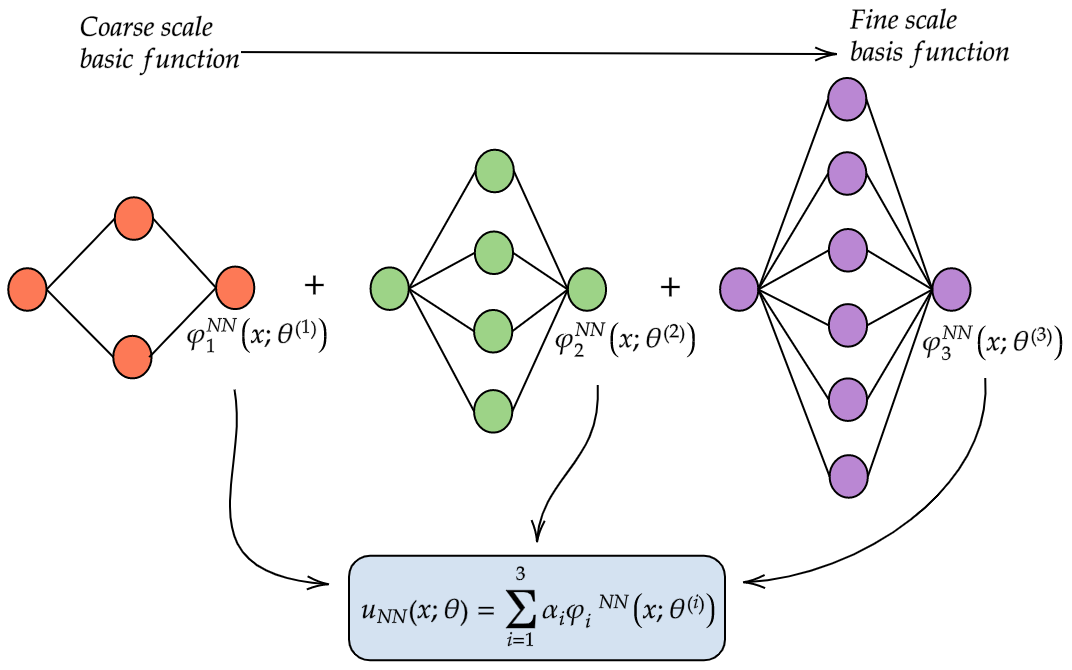
Main Idea. Galerkin neural networks seeks to approximate the solution \(u\) of \eqref{eq:variational} by projecting it onto a finite-dimensional subspace whose basis functions are outputs of a sequence of shallow neural networks. That is, we approximate \(u\) with
\[\begin{align} u_{NN}(x;\theta) \approx \sum_{i=1}^{m} \alpha_{i} \varphi_{i}^{NN}(x;\theta^{(i)}). \end{align}\]With this idea in mind, it all boils down to how to generate the basis functions \(\{\varphi_{i}\}_{i=1}^{m}\), since once we have the basis functions in hand, we simply follow \eqref{eq:discrete} to obtain the coefficients \(\alpha\).
Figure 3 provides a visualization of the overall idea. You’ll notice I’ve labeled the basis function coming from the smallest network as the “coarse scale” basis function while the one coming from the widest network is labeled a “fine scale” basis function. This has to do with how we can interpret the basis functions and I’ll discuss this more once we’ve actually covered how to generate the basis functions.
And the way that we’re going to generate these basis functions has to do with learning Riesz representations of something called the weak residual. Let’s suppose we start off with some initial approximation \(u_{0} \in X\) to the true solution \(u\). I want to emphasize here that \(u_{0}\) can be any element of \(X\). In our paper, we always made the choice \(u_{0} = 0\) in the examples, which is just to say that we don’t have to have any prior knowledge of the solution at all to pick \(u_{0}\).
Definition. Given \(u_{0} \in X\), the weak residual of \(u_{0}\) with respect to \eqref{eq:variational} is the linear functional \(r(u_{0}) : X \to \mathbb{R}\) given by
\[\begin{align} \langle r(u_{0}),v \rangle = L(v) - a(u_{0},v).\label{eq:weak residual} \end{align}\]The notation \(\langle r(u_{0}),v \rangle\) denotes the evaluation of \(r(u_{0})\) at \(v\). The quantity \eqref{eq:weak residual} will be zero by definition if \(u_{0}\) is the true solution. Otherwise, it is just a nonzero number.
I. Riesz Representation of Weak Residuals
We note that \(L(v) = a(u,v)\) by \eqref{eq:variational}, so we can rewrite \eqref{eq:weak residual} as
\[\langle r(u_{0}),v \rangle = a(u,v) - a(u_{0},v) = a(u-u_{0},v). \label{eq:weak residual riesz}\]Rewriting it in this way allows us to make some observations on \(r(u_{0})\).
Theorem (Riesz representation). Let \(X\) be a Hilbert space with norm \(\|\cdot\|_{X}\) and inner product \((\cdot,\cdot)_{X}\) and let \(L : X \to \mathbb{R}\) be a bounded linear functional on \(X\). There exists an element \(\varphi_{L} \in X\) such that
\[\langle L,v \rangle = (\varphi_{L},v)_{X}\]for all \(v \in X\). Moreover, we have \(\|L\|_{*} = \|\varphi_{L}\|_{X}\), where \(\|\cdot\|_{*}\) denotes the operator norm.
The Riesz representation theorem says that in a Hilbert space, linear functionals can be “identified” with elements of the Hilbert space itself. Namely, if we want to evaluate a linear functional \(L\) for some argument \(v\), this is equivalent to taking the inner product of \(v\) with some element \(\varphi_{L} \in X\). This kernel \(\varphi_{L}\) is known as the Riesz representation of \(L\).
This suggests that the Riesz representation of the functional \(r(u_{0})\) is the error \(u-u_{0}\), at least when we consider the norm on \(X\) to be defined by \(\|\cdot\|_{X} := a(\cdot,\cdot)^{1/2}\) (this definition of \(\|\cdot\|_{X}\) means that \((\cdot,\cdot)_{X} := a(\cdot,\cdot)\)). We can define the norm and inner product on \(X\) in this way if \(a\) is symmetric and positive-definite, so for now we’re going to assuming that \(a\) is symmetric positive-definite. The norm that’s induced by the operator \(a\) has a special name: the energy norm. It’s standard to use triple bars to denote this norm: \(\vert\vert\vert \cdot \vert\vert\vert := a(\cdot,\cdot)^{1/2}\).
Thus, we can explicitly say what the Riesz representation of the weak residual is, but who cares? Why is this important? Let’s introduce the variable \(\varphi\) to denote the normalized Riesz representation of \(r(u_{0})\), i.e. \(\varphi = (u-u_{0})/\vert\vert\vert u-u_{0} \vert\vert\vert\). Now suppose we could compute this \(\varphi\). Then we could easily take a linear combination \(\beta_{0}u_{0} + \beta_{1}\varphi\) and recover the true solution – just take \(\beta_{0} = 1\) and \(\beta_{1} = \vert\vert\vert u-u_{0} \vert\vert\vert\).
But typically, we won’t be able to compute \(\varphi\) exactly. This is akin to solving \eqref{eq:variational} exactly, which can only be done in very simple cases. Otherwise, we’ll have to approximate \(\varphi\), and the key to doing this is actually a very simple property of the Riesz representation of the weak residual.
Proposition 1. Let \(\varphi := (u-u_{0})/\vert\vert\vert u-u_{0} \vert\vert\vert\) denote the normalized Riesz representation of \(r(u_{0})\). Then \(\varphi\) satisfies
\[\begin{align} \varphi = \text{argmax}_{v \in X \cap B} \langle r(u_{0}),v \rangle, \;\;\;B := \{v \in X : \vert\vert\vert v \vert\vert\vert = 1\} \label{eq:continuous maximizer} \end{align}\]Proposition 1 says that the normalized Riesz representation \(\varphi\) is actually the maximizer of the weak residual over all elements of \(X\) with unity energy norm. In theory, all we need to do to compute \(\varphi\) is solve the maximization problem laid out in \eqref{eq:continuous maximizer}. We already know we can’t solve this maximization problem over all of \(X\) (which is infinite-dimensional). Instead, what if we replace \(X\) with the set of all functions that can be represented by a particular neural network architecture?
II. Learning a Basis Function
Let’s define the set \(V_{n}^{\sigma}\) to be the set of all functions which can be realized by a feedforward neural network with a single hidden layer of \(n\) neurons and activation function \(\sigma\):
\[\begin{align} V_{n}^{\sigma} := \left\{ v : v(x) = \sum_{i=1}^{n} c_{i}\sigma(x\cdot W_{i} + b_{i}), \;W \in \mathbb{R}^{d\times n}, \;b \in \mathbb{R}^{1\times n}, \;c \in \mathbb{R}^{n} \right\}.\label{eq:Vn} \end{align}\]And let’s replace \(X \cap B\) in \eqref{eq:continuous maximizer} with \(V_{n}^{\sigma} \cap B\). We’ll call the maximizer of this problem \(\varphi_{1}^{NN}\):
\[\begin{align} \varphi_{1}^{NN} = \text{argmax}_{v \in V_{n}^{\sigma} \cap B} \langle r(u_{0}),v(\cdot;\theta) \rangle. \label{eq:discrete maximizer} \end{align}\]The maximization problem in \eqref{eq:discrete maximizer} is now tractable. In fact, we can approximate it using the typical optimizers we would use for other deep learning problems. Before we go and do this though, we would do well to quantify how far off \(\varphi_{1}^{NN}\) is from the true Riesz representation \(\varphi\).
Theorem 1. Given \(\varepsilon \in (0,1)\), there exists \(n \in \mathbb{N}\) and \(\varphi_{1}^{NN} \in V_{n}^{\sigma} \cap B\) defined by \eqref{eq:discrete maximizer} such that \(\begin{align} \vert\vert\vert \varphi-\varphi_{1}^{NN} \vert\vert\vert \leqslant \frac{2\varepsilon}{1-\varepsilon}. \end{align}\)
The proof is somewhat technical and provided in [2]. It piggybacks off of standard universal approximation results such as those of Cybenko, Hornik, and Leshno. As such, Theorem 1 doesn’t quantify how the error converges with respect to the degrees of freedom in the network (such as in \eqref{eq:linear interp}).
As an aside, it’s worth noting that there have been recent efforts to quantify both the minimum width and depth of a neural network necessary to reach a target accuracy, and how the approximation error in neural networks varies with respect to the width and depth of the network a la \eqref{eq:linear interp}. Some examples of this are the excellent work of De Ryck, Lanthaler, and Mishra; Yarotsky; and Opschoor, Petersen, and Schwab. Such results can be integrated with Theorem 1 when appropriate to obtain explicit error bounds for our method.
Once we have \(\varphi_{1}^{NN}\) computed (see \(\S\)4.IV for implementation details), we can use it to “correct” the initial approximation \(u_{0}\). Let’s form the two-dimensional subspace \(S_{1} := \text{span}\{u_{0}, \varphi_{1}^{NN}\}\) and use Galerkin’s method to project \(u\) onto \(S_{1}\):
\[\begin{align} u_{1} \in S_{1} \;:\; a(u_{1},v) = L(v) \;\;\;\forall v \in S_{1}.\label{eq:S1} \end{align}\]\eqref{eq:S1} is equivalent to solving a \(2\times 2\) linear system to obtain \(u_{1} = \alpha_{0}u_{0} + \alpha_{1}\varphi_{1}^{NN}\). We can derive an error estimate for \(u_{1}\) based on Theorem 1.
Theorem 2. Given \(\varepsilon \in (0,1)\) and \(\varphi_{1}^{NN}\) as defined in \eqref{eq:discrete maximizer}, there holds
\[\begin{align} \vert\vert\vert u-u_{1} \vert\vert\vert \leqslant \frac{2\varepsilon}{1-\varepsilon} \vert\vert\vert u-u_{0} \vert\vert\vert. \end{align}\]This result says that if we supplement the initial approximation \(u_{0}\) with the approximate Riesz representation \(\varphi_{1}^{NN}\), we should expected to reduce the error in the initial approximation by a factor of ~\(\varepsilon\).
Remark. Theorems 1 and 2 only quantify the approximation error accrued when using the set \(V_{n}^{\sigma}\) as a stand-in for the infinite-dimensional space \(X\). Error in the optimization method used to compute \eqref{eq:discrete maximizer} is another significant source of error. Eventually stagnation of these methods is ubiquitous in deep learning. Galerkin neural networks addresses this issue by conceding that we won’t be able to use a single large DNN to capture all features of the solution. Rather, we sequentially compute basis functions as corrections to the error accrued in the previous steps in order to improve accuracy incrementally.
III. Adaptive Subspace Generation
We now have an improved approximation \(u_{1}\), but what if this still isn’t good enough? We can naturally iterate the procedure thus far to generate more basis functions. This is done by replacing \(r(u_{0})\) with \(r(u_{1})\) and computing its maximizer in \(V_{n}^{\sigma} \cap B\). To generalize, the \(i\)th basis function \(\varphi_{i}^{NN}\) is generated by computing
\[\begin{align} \varphi_{i}^{NN} = \text{argmax}_{v \in V_{n_{i}}^{\sigma} \cap B} \langle r(u_{i-1}),v \rangle.\label{eq:basis function i} \end{align}\]We’re using \(n_{i}\) here to denote the width of the neural network for \(\varphi_{i}^{NN}\). The \(i\)th approximation \(u_{i}\) is computed by forming the subspace \(S_{i} := \text{span}\{u_{0}, \varphi_{1}^{NN}, \dots, \varphi_{i}^{NN}\}\) and solving
\[\begin{align} u_{i} \in S_{i} \;:\; a(u_{i},v) = L(v) \;\;\;\forall v \in S_{i}.\label{eq:ui} \end{align}\]Corollary 1. Given \(0 < \varepsilon_{i} < 1\), \(\varphi_{i} := (u-u_{i-1})/\vert\vert\vert u-u_{i-1} \vert\vert\vert\), \(\varphi_{i}^{NN}\) defined by \eqref{eq:basis function i}, and \(u_{i}\) defined by \eqref{eq:ui}, there holds
\[\begin{align} \vert\vert\vert \varphi_{i} - \varphi_{i}^{NN} \vert\vert\vert \leqslant \frac{2\varepsilon_{i}}{1-\varepsilon_{i}} \end{align}\]and \(\begin{align} \vert\vert\vert u-u_{i} \vert\vert\vert \leqslant \prod_{j=1}^{i}\frac{2\varepsilon_{j}}{1-\varepsilon_{j}} \vert\vert\vert u-u_{0} \vert\vert\vert. \end{align}\)
Each basis function \(\varphi_{i}^{NN}\) approximates the Riesz representation \(\varphi_{i}\) of the \(i\)th weak residual, which shouldn’t be too surprising. The approximation \(u_{i}\) is exponentially convergent with respect to the number of basis functions, and in fact each basis function added to the subspace \(S_{i}\) reduces the original error \(\vert\vert\vert u-u_{0} \vert\vert\vert\) by a factor of ~\(\varepsilon_{i}\).
We could go on generating these basis functions indefinitely. For problems where we have access to the true solution, we could compute exact errors of our approximation to determine when to stop adding basis functions to the subspace. For most realistic problems though, we won’t have access to such metrics and will need to estimate the error on the fly. Conveniently, Galerkin neural networks has a very nice way to do this.
We already know that the Riesz representation \(\varphi_{i}\) is the maximizer of \(r(u_{i-1})\). More importantly, the maximum value of \(r(u_{i-1})\) is actually the energy error \(\vert\vert\vert u-u_{i-1} \vert\vert\vert\):
\[\vert\vert\vert u-u_{i-1} \vert\vert\vert = \max_{v\in V_{n_{i}}^{\sigma} \cap B} \langle r(u_{i-1}),v \rangle = \langle r(u_{i-1}),\varphi_{i} \rangle.\]Thus, when replacing \(\varphi_{i}\) with \(\varphi_{i}^{NN}\), it is reasonable to expect \(\langle r(u_{i-1}),\varphi_{i}^{NN} \rangle \approx \vert\vert\vert u-u_{i-1} \vert\vert\vert\). We can quantify just how well the weak residual approximates the energy norm with the following result.
Theorem 3. Given \(\varepsilon_{i} \in (0,1/3)\), there holds
\[\begin{align} \frac{1-\varepsilon_{i}}{1+\varepsilon_{i}} \langle r(u_{i-1}),\varphi_{i}^{NN} \rangle \leqslant \vert\vert\vert u-u_{i-1} \vert\vert\vert \leqslant \frac{1-\varepsilon_{i}}{1-3\varepsilon_{i}} \langle r(u_{i-1}),\varphi_{i}^{NN} \rangle. \end{align}\]This says that if we evaluate the residual \(r(u_{i-1})\) at the computed basis function \(\varphi_{i}^{NN}\), it should be a reasonable a posteriori estimate of the energy error, which is typically a physical quantity of interest!
In effect, this means we can choose a desired tolerance \(\texttt{tol}\) and use \(\langle r(u_{i-1}),\varphi_{i}^{NN} \rangle < \texttt{tol}\) as a stopping ctierion for determining when to stop generating new basis functions.
i. An Illustrative Example
Before discussing the finer details of implementation and showcasing some broader examples, I want to provide a straightforward one-dimensional example which demonstrates all of the key features of Galerkin neural networks. Let’s consider the Poisson equation:
\[\begin{align} \begin{cases} -u''(x) = f(x) &\text{in}\;(0,1)\\ u(0) - \tau u'(0) = 0\\ u(1) + \tau u'(1) = 0. \end{cases}\label{eq:poisson1d} \end{align}\]The parameter \(\tau \ll 0\) is designed to approximate a homogeneous Dirichlet boundary condition: as \(\tau \to 0\), the solution of the above BVP converges to the solution when \(\tau = 0\). The reason for having this parameter is due to the fact that weak formulations of this problem typically contain information about the boundary condition in the Hilbert space \(X\), e.g. in \eqref{eq:poisson1d weak} we had \(X=H^{1}_{0}(0,1)\), but in general the Galerkin neural network basis functions \(\varphi_{i}^{NN}\) won’t be in \(H^{1}_{0}(0,1)\), only \(H^{1}(0,1)\).
The variational formulation for \eqref{eq:poisson1d} is
\[\begin{align} u \in H^{1}(0,1) \;:\; a(u,v) :&= (u',v')_{L^{2}} + \frac{1}{\tau}u(0)v(0) + \frac{1}{\tau}u(1)v(1)\notag\\ &= (f,v)_{L^{2}} =: L(v) \;\;\;\;\;\;\;\;\;\;\;\;\;\;\;\;\;\;\;\;\;\;\;\;\forall v \in H^{1}(0,1).\notag \end{align}\]We’ll take \(f(x) = (2\pi)^{2}\sin(2\pi x) + (4\pi)^{2}\sin(4\pi x) + (6\pi)^{2}\sin(6\pi x)\) in which case the true solution \(u\) is
\[\begin{align} u(x) = \sin(2\pi x) + \sin(4\pi x) + \sin(6\pi x) + \frac{-24\tau\pi x + 12\pi\tau}{1+2\tau}.\notag \end{align}\]I’ll show first what the Riesz representations and basis functions look like. The different parameters used in this example are provided in Table 2.
\(\small \begin{array}{c|c|c|c|c|c|c} \hline \textbf{Parameter} & u_{0} & \text{widths } n_{i} & \text{activation} & \text{optimizer} & \text{learn rate} & \text{training set}\\ \hline \textbf{Value} & \equiv 0 & 5\cdot 2^{i-1} & \tanh((1+i)t) & \text{Adam} & 10^{-2}/1.1^{i-1} & 512 \text{ GL pts} \\ \hline \end{array}\)
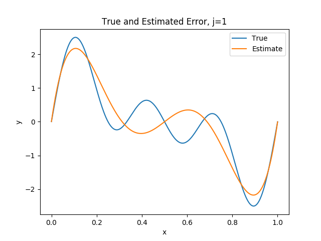
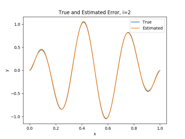


One striking observation is that the first couple of Riesz representations consist of mainly low frequency oscillations while the later Riesz representations consist of very high frequency oscillations, and generally speaking each Riesz representation is mono-frequency. Thus, Galerkin neural networks essentially decomposes the problem into a series of subproblems, each of which encodes different frequencies of the solution. We also observe that each neural network is able to very closely approximate the true Riesz representation (granted, this is a very simple problem).
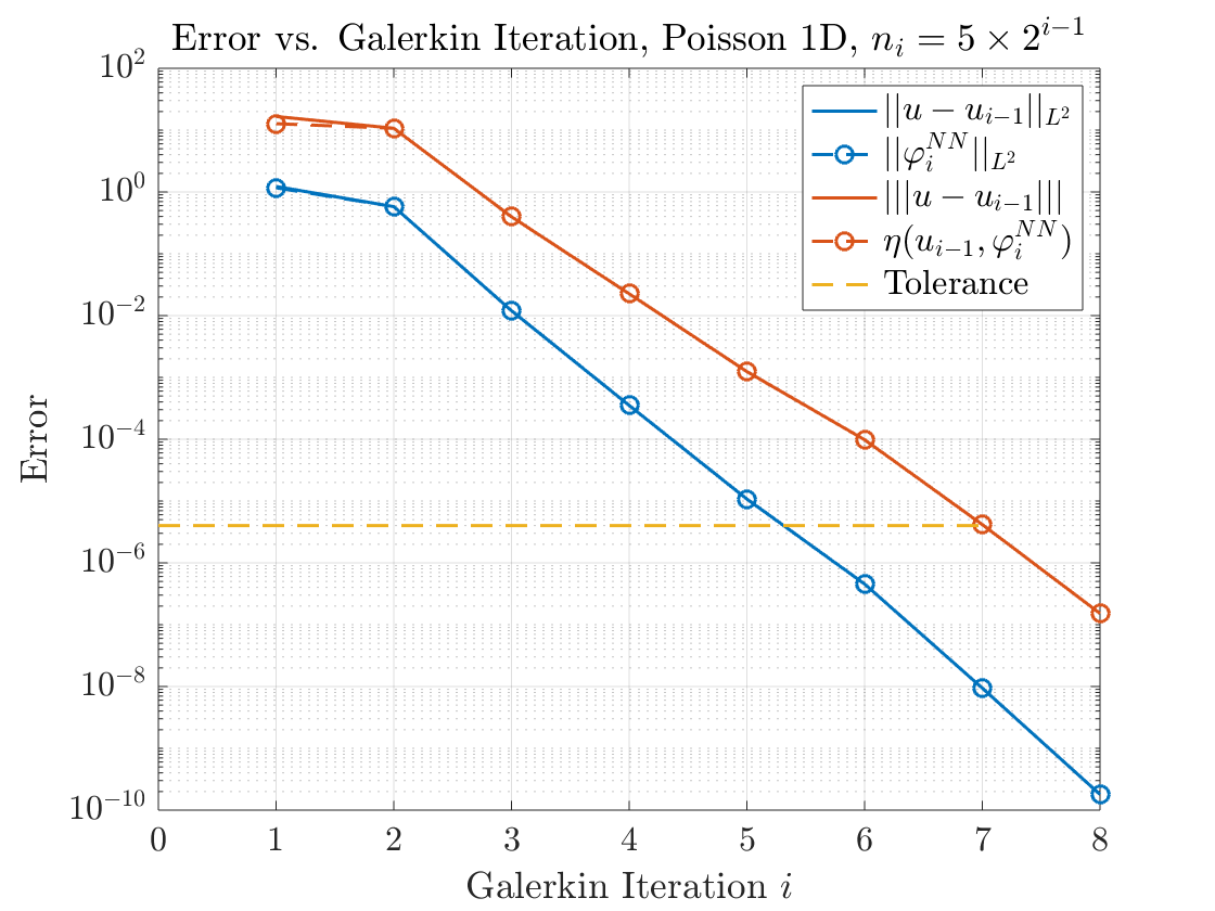
Utilizing all of these basis functions to approximate the solution results in a highly accurate approximation as seenin Figure 5 (\(\eta(u_{i-1}, \varphi_{i}^{NN})\) was the notation we used in [2] to denote the weak residual). As predicted by Theorem 3, the weak residual almost perfectly approximates the energy error \(\vert\vert\vert u-u_{i-1} \vert\vert\vert\). Similarly, we can actually take \(\vert\vert \varphi_{i}^{NN} \vert\vert_{L^{2}}\) as an approximation to the \(L^{2}\) error, which is pretty accurate as well. It’s also clear that with each basis function added to the subspace, we reduce the approximation error by a fixed amount (Corollary 1).
IV. Implementation Details
Before moving on to some more examples, I’ll touch of some implementation details in this section. The first order of business is how to actually compute \eqref{eq:discrete maximizer}. Rather than seeking a normalized maximizer, we divide through by the energy norm:
\[\begin{align} \text{argmax}_{v \in V_{n}^{\sigma} \cap B} \langle r(u_{i-1}),v \rangle &= \text{argmax}_{v \in V_{n}^{\sigma}} \frac{\langle r(u_{i-1}),v \rangle}{\vert\vert\vert v \vert\vert\vert}\notag\\ &= \text{argmax}_{\theta} \frac{\langle r(u_{i-1}),v(\cdot;\theta) \rangle}{\vert\vert\vert v(\cdot;\theta) \vert\vert\vert}\notag \end{align}\]Next, we note that \(\langle r(u_{i-1}),v \rangle\) consists of many inner products (integrals) which must be evaluated. We will approximate these integrals with standard Gaussian quadrature rules. To be concrete, let’s consider the 1D Poisson example from the previous section. A quadrature rule consists of a set of nodes \(\{x_{i}\}_{i=1}^{n_{g}} \subset \Omega\) and weights \(\{w_{i}\}_{i=1}^{n_{g}}\) which are used to approximate the integral as a weighted sum of function evaluations over the nodes:
\[\int_{\Omega} g(x)\;dx \approx \sum_{i=1}^{n_{g}} w_{i}g(x_{i}).\]For the 1D Poisson example, the weak residual is approximated by
\[\begin{align} \frac{\langle r(u_{i-1}),v \rangle}{\vert\vert\vert v \vert\vert\vert} &\approx \frac{L_{1} - L_{2} - L_{3}}{(\sum_{j=1}^{n_{g}} w_{j}v'(x_{j};\theta)^{2} + \tau^{-1}[v(0;\theta)^{2} + v(1;\theta)^{2}])^{1/2}}\notag\\ L_{1} &= \sum_{j=1}^{n_{g}} w_{j}f(x_{j})v(x_{j};\theta)\notag\\ L_{2} &= \sum_{j=1}^{n_{g}} w_{j}u'_{i-1}(x_{j})v'(x_{j};\theta)\notag\\ L_{3} &= \tau^{-1}[u_{i-1}(0)v(0;\theta) + u_{i-1}(1)v(1;\theta)].\notag \end{align}\]For all examples here, we use a Gauss-Legendre quadrature rule in which the nodes and weights are obtained from Legendre polynomials.
To perform the numerical optimization, we use a hybrid first-order least squares optimization approach. This approach considers the weights of the activation layer (i.e. the parameters \(c\) in \eqref{eq:Vn}) to be expansion coefficients of the nonlinear basis \(\sigma\). It’s similar in concept to nonlinear least squares methods such as Levenberg-Marquardt which obtain \(c\) by solving a linear least squares system.
In [2] we proposed the following training procedure. We update the hidden parameters using a gradient-based optimizer such as gradient descent:
\[\begin{align} W &\leftarrow W + \lambda \nabla_{W}\left[ \frac{\langle r(u_{i-1}),v(\cdot;\theta) \rangle}{\vert\vert\vert v(\cdot;\theta) \vert\vert\vert} \right]\notag\\ b &\leftarrow b + \lambda \nabla_{b}\left[ \frac{\langle r(u_{i-1}),v(\cdot;\theta) \rangle}{\vert\vert\vert v(\cdot;\theta) \vert\vert\vert} \right].\notag\\ \end{align}\]The linear parameters are updated according to the least squares solve:
\[\begin{align} \begin{cases} c \leftarrow \text{argmin}_{c \in \mathbb{R}^{n}} \|Ac-F\|_{\ell^{2}}\notag\\ A_{k\ell} = a(\sigma_{k}, \sigma_{\ell}), \;\;\;F_{k} = L(\sigma_{k}) - a(u_{i-1},\sigma_{k})\\ \sigma_{k} := \sigma((\cdot)\cdot W_{k} + b_{k}). \end{cases} \end{align}\]This linear system is equivalent to taking the orthogonal projection of the Riesz representation \(u-u_{i-1}\) with respect to \(a(\cdot,\cdot)\) onto the space \(\text{span}\{\sigma(x\cdot W_{i}+b_{i})\}_{i=1}^{n}\).
Lastly, there is the matter of how to initialize the parameters \(W\) and \(b\). In computer vision applications, it’s common to draw values of \(W\) and \(b\) from a probability distribution (often uniform or Gaussian with mean and variance depending in some way on the width of the layer). These initializers are sometimes not optimal for function and PDE approximation. In [3], the authors propose a new initializer (the “box initialization”) which distributes the hyperplanes of the network more evenly throughout the computational domain \(\Omega\). While this initialization was developed for very deep ResNets, it is sufficient for our very shallow networks.

A full implementation (using Google’s Jax framework) for some simple 1D and 2D problems is provided on my GitHub. The rest of this post will be dedicated to showcasing more numerical examples.
5. Numerical Examples
I. Approximation of a Nonsmooth Function
The next example we’ll look at is a two-dimensional function approximation problem. Suppose we have target data \(f \in L^{2}(\Omega)\) and wish to fit this function with a neural network. The variational formulation for this problem is
\[\begin{align} u \in L^{2} \;:\; a(u,v) := (u,v)_{L^{2}} = (f,v)_{L^{2}} =: L(v) \;\;\;\forall v \in L^{2}, \end{align}\]which is essentially just an \(L^{2}\) projection. The data \(f\) for this example will be space-time data describing the volume fraction of spherical particles in a suspension flow. Figure 4 shows the target function \(f\) that we’re going to approximate with Galerkin neural networks.
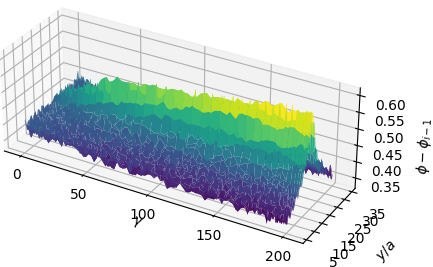
This data was generated using something called the force-coupling method with data provided by Amanda Howard. The application of Galerkin neural networks to this problem was carried out during my time as an intern at Pacific Northwest National Laboratory. The precise details of the force-coupling method aren’t important for demonstrating the main ideas of Galerkin neural networks.
The different parameters used in this simulation are provided in Table 2.
\(\small \begin{array}{c|c|c|c|c|c|c} \hline \textbf{Parameter} & u_{0} & \text{widths } n_{i} & \text{activation} & \text{optimizer} & \text{learn rate} & \text{training set}\\ \hline \textbf{Value} & \equiv 0 & 20\cdot 2^{i-1} & \tanh((1+1.25i)t) & \text{Adam} & 10^{-2}/1.1^{i-1} & 128\times 128 \text{ GL pts} \\ \hline \end{array}\)
I’ll first show the exact Riesz representations for the first two residuals (\(\varphi_{1}\) and \(\varphi_{2}\)) as well as their neural network approximations (\(\varphi_{1}^{NN}\) and \(\varphi_{2}^{NN}\)).
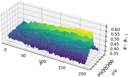
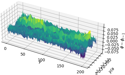

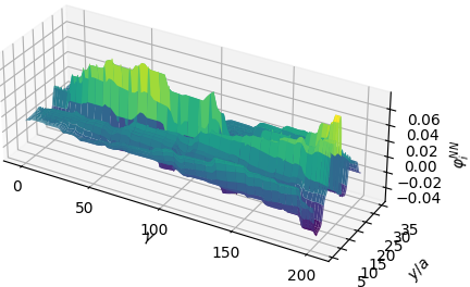
What we observe is that the first basis function \(\varphi_{1}^{NN}\) is a very coarse approximation to the true Riesz representation. It captures the low frequency behavior and “sees” that the Riesz representation is a symmetric function about the \(y\)-centerline but otherwise misses all of the fine-scale behavior. The same is true for \(\varphi_{2}^{NN}\) which essentially looks like a smoothed out version of \(\varphi_{2}\), albeit containing higher frequencies than \(\varphi_{1}^{NN}\).
Let’s take a look at the next couple of Riesz representations and their approximations.
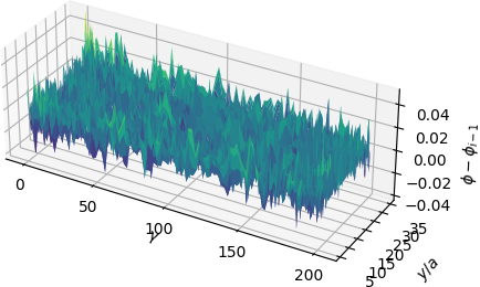
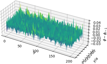
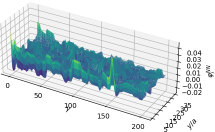
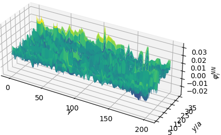
We observe that \(\varphi_{3}\) and \(\varphi_{4}\) encode higher frequency behavior of the error. In all of these basis functions however, it’s clear that we never approximate the true Riesz representations perfectly. Indeed, the first couple of basis functions don’t look very good at all. Each basis function is only meant to reduce particular frequencies in the error, much like in the first example.
When we take a linear combination of these basis functions, we can see more clearly the effect each one has on the overall approximation.
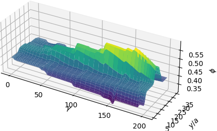
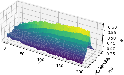
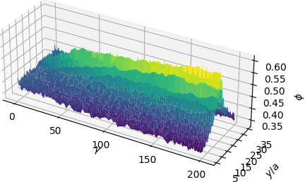
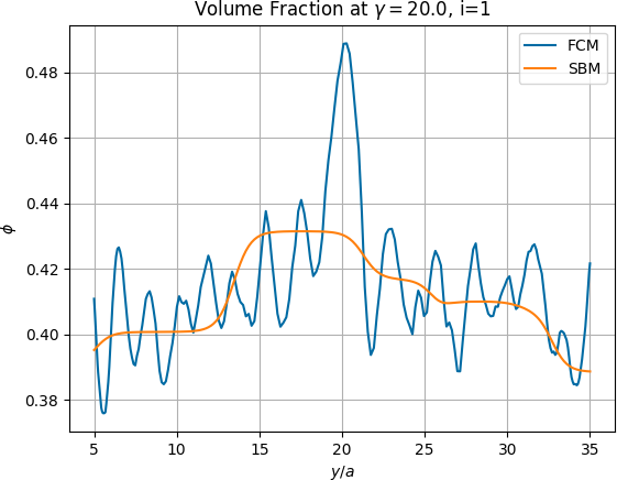
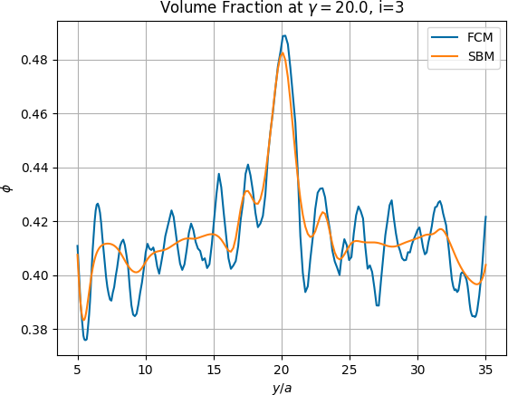

A common question I get asked during conference talks (and more recently, job talks) is what happens if we only use the widest neural network in our sequence to approximate the solution. The width of the network for \(\varphi_{i}^{NN}\) is \(n_{i}=20\times 2^{i-1}\) for this example, so \(u_{7}\) which utilizes networks of widths 20, 40, 80, 160, 320, 640, and 1280 to approximate the component basis functions. If we generate only a single basis function coming from a network with width \(n_{1}=1280\), we don’t come close to approximating the target function to the same degree of accuracy obtained from the full ensemble of basis function.
The analogous result using a single wide neural network is shown in Figure 7. While \(\varphi_{1}^{NN} \in V_{1280}^{\sigma}\) is certainly more accurate than \(\varphi_{1}^{NN} \in V_{20}^{\sigma}\) (the initial results shown in Figure 6), it’s clear that the former doesn’t come close to the accuracy obtained by using seven basis functions, the last of which comes from \(\varphi_{7}^{NN} \in V_{1280}^{NN}\). Sure, we can add a second basis function, say \(\varphi_{2}^{NN} \in V_{2560}^{NN}\) if we continue with the same rule for the network widths, but this is computationally inefficient.
I’ll discuss computational costs more in \(\S\)4.IV, but roughly speaking, the computational cost for Galerkin neural networks is on the same order as the computational cost of computing the basis function coming from the widest network. This means that computing \(\varphi_{1}^{NN} \in V_{1280}^{\sigma}\) takes about the same amount of time as \(\varphi_{7}^{NN} \in V_{1280}^{NN}\) and yet is several orders of magnitude less accurate. All this to say that the coarse basis functions we learn initially are important! It might not seem like it since the initial basis functions aren’t great approximations to their respective Riesz representations (Figure 5), but they encode the lower frequencies of the solution and allow the later basis functions to focus on higher frequencies.


II. Poisson Equation with Line Source Data
The last example I want to showcase is one which contains singular data. We take
\[L(v) = \int_{\Gamma} v\;ds, \;\;\;\Gamma := \{ (x,y) : x^{2} + y^{2} = R_{0}^{2} \}.\]\(L\) corresponds to a Dirac-delta distribution over a circle, and the weak solution to the problem
\[u \in H^{1}(\Omega) \;:\; (\nabla u, \nabla v)_{L^{2}(\Omega)} + \frac{1}{\tau}(u,v)_{L^{2}(\partial\Omega)} = L(v) \;\;\;\forall v \in H^{1}(\Omega)\]in the domain \(\Omega = \{(x,y) : x^{2}+y^{2} = R_{e}^{2}\}\) is
\[u(r,\theta) = -\dfrac{\tau}{R_{0}\log(R_{0}/R_{e})} + \begin{cases} 1, &r \leqslant R_{0}\\ \dfrac{1}{\log(R_{0}/R_{e})}\log(r/R_{e}), &R_{0} \leqslant r \leqslant R_{e}. \end{cases}\]The parameters used for this example are given in Table 4 and the results in Figure 11.
\(\small \begin{array}{c|c|c|c|c|c|c} \hline \textbf{Parameter} & u_{0} & \text{widths } n_{i} & \text{activation} & \text{optimizer} & \text{learn rate} & \text{training set}\\ \hline \textbf{Value} & \equiv 0 & 30\cdot 2^{i-1} & \tanh((1+i)t) & \text{Adam} & 2\cdot 10^{-2}/1.1^{i-1} & \begin{array} 128\times 128 \text{ GL pts in }\Omega\\ 512 \text{ equally spaced on }\partial\Omega \text{ and }\Gamma \end{array} \\ \hline \end{array}\)


We observe that we’re able to accurately capture the corner in the solution that appears along \(\Gamma\). Moreover, even for this reduced regularity problem, we observe convergence at a fixed rate as the theory suggests. This rate of convergence is slower due to the reduced regularity as one might also expect. In the presence of singular behavior, there are several approaches to improve convergence. The first is to use a smarter formulation of the problem designed to better capture these features. An example of this can be found in our follow-up work, Galerkin neural network approximation of singularly-perturbed elliptic systems (preprint can be found here). The second is to utilize activation functions and/or a choice of \(u_{0}\) which capture the singular behavior. In the case of boundary layers, corner singularities, etc. much is known about the structure of solutions in the vicinity of these features and is readily available in the literature. Our current work focuses on such approaches.
6. Key Takeaways
Galerkin neural networks approximate the solution of a PDE by expressing it as the sum of several shallow neural networks, each of which encode features of different frequencies. The result is an approximation that is more than the sum of its parts would suggest, as using only the most expressive network in the sequence is unable to come close to replicating the same result.
There are many papers out there purporting to combine Galerkin methods with neural networks yet neither use a Galerkin method nor benefit from any of its properties. We leveraged the nice approximation properties of Galerkin methods with the expressivity of neural networks in a way that feels true to the source material and performs well for a number of difficult test problems.
I hope you found this post informative. If you’re interested in trying out this method for yourself, feel free to check out the GalerkinNN repo on GitHub.
References
[1] Dissanayake, M. and N. Phan-Thien. “Neural network-based approximations for solving partial differential equations.” Communications in Numerical Methods in Engineering, 10(3), 195-201.
[2] Ainsworth, M. and J. Dong (2021). “Galerkin neural networks: a framework for approximating variational equations with error control.” SIAM Journal on Scientific Computing, 43(4), A2474-A2501.
[3] Cyr, E. C., Gulian, M. A., Patel, R. G., Perego, M., and N. A. Trask (2020). Robust training and initialization of deep neural networks: An adaptive basis viewpoint. In Mathematical and Scientific Machine Learning (pp. 512-536). PMLR.
Codes & Resources
- GalerkinNN repository on GitHub
- All figures in this post were generated by me unless otherwise noted.