Numerical methods for conservation laws -- high-order finite volume methods and slope limiters (part 2)
1. High Order Finite Volume Methods
Last time, we established that the explicit first order finite volume scheme is given by \(\begin{equation} \bar{u}_{j}^{n+1} = \bar{u}_{j}^{n} - \frac{\Delta t}{\Delta x}\left( \hat{f}(\bar{u}_{j}^{n}, \bar{u}_{j+1}^{n}) - \hat{f}(\bar{u}_{j-1}^{n}, \bar{u}_{j}^{n}) \right), \label{eq:finitevol2} \end{equation}\)
where \(\bar{u}_{j}^{n}\) denotes the cell averages at time \(t^{n}\) and \(\bar{u}_{j}^{n+1}\) the cell averages at time \(t^{n+1} = t^{n} + \Delta t\). Here, \(\hat{f}\) is the numerical flux function which takes as inputs cell averages and returns an approximation of the flux function at the cell endpoints \(x_{j+1/ 2}\), i.e. \(f(u_{j+1/ 2}) \approx \hat{f}(\bar{u}_{j}, \bar{u}_{j+1})\) and \(f(u_{j-1/ 2}) \approx \hat{f}(\bar{u}_{j-1}, \bar{u}_{j})\).
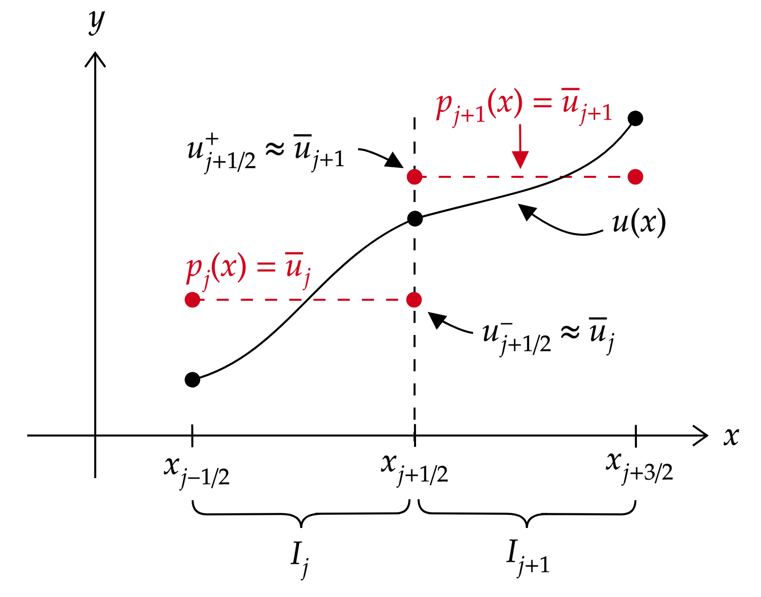
More generally, we can view the quantity \(\bar{u}_{j}\) as a first order (zero degree polynomial) reconstruction of \(u(x)\) in cell \(I_{j}\) using the cell average. The same can be said of \(\bar{u}_{j+1}\) in cell \(I_{j+1}\). By approximating \(u(x_{j+1/ 2}^{-}) = u_{j+1/ 2}^{-} \approx \bar{u}_{j}\) on the left “side” of \(x_{j+1/ 2}\) and \(u(x_{j+1/ 2}^{+}) = u_{j+1/ 2}^{+} \approx \bar{u}_{j+1}\) on the right side of \(x_{j+1/ 2}\), the numerical flux has a natural interpretation as \(f(u_{j+1/ 2}) \approx \hat{f}(u_{j+1/ 2}^{-}, u_{j+1/ 2}^{+})\). We reconcile the two reconstructions at \(x_{j+1/ 2}\) by utilizing the numerical flux function. Figure 1 illustrates this concept.
I. Polynomial Reconstruction
Viewing the finite volume scheme as a reconstruction procedure using the cell averages is key to developing higher order methods. Using \eqref{eq:finitevol2}, we have \(u_{j+1/ 2}^{-} = \bar{u}_{j} + \mathcal{O}(\Delta x)\). Suppose we want to develop a third-order finite volume scheme now. In particular, we would like to have
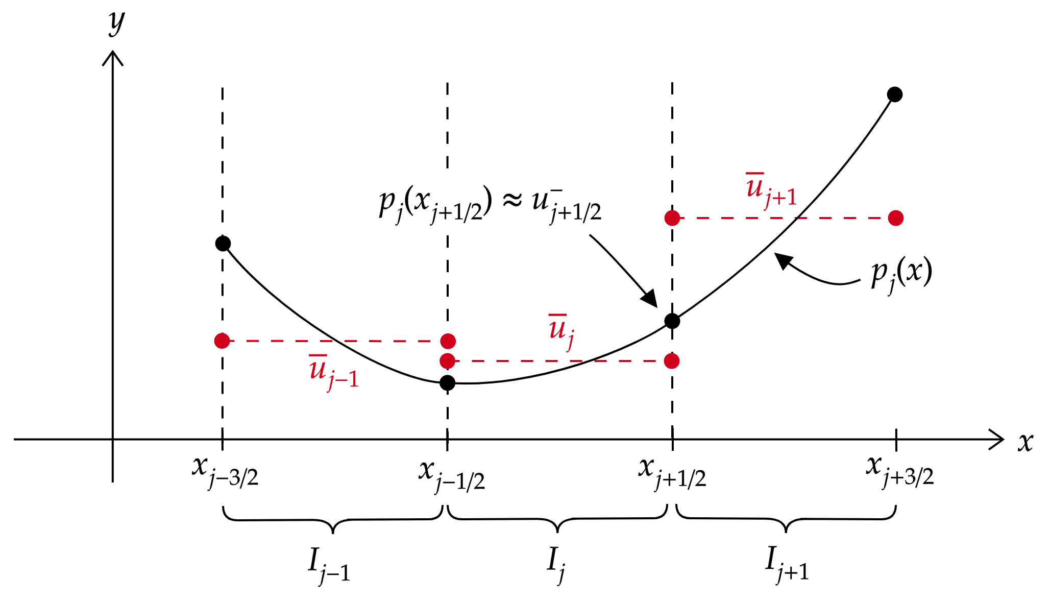
\[u_{j+1/ 2}^{-} = \mathcal{F}(\bar{u}_{j-p}, \dots, \bar{u}_{j+q}) + \mathcal{O}(\Delta x^{3}),\]where \(p\) and \(q\) are integers to be chosen by us. It stands to reason that if we want a third-order reconstruction of $u(x)$ in cell \(I_{j}\), we need to use three “pieces” of information: \(u_{j+1/ 2}^{-} \approx \mathcal{F}(\bar{u}_{j-1}, \bar{u}_{j}, \bar{u}_{j+1})\). In other words, we are seeking a degree two polynomial \(p_{j}(x) = ax^{2} + bx + c\) in \(I_{j}\) such that \(u_{j+1/ 2}^{-} = p_{j}(x_{j+1/ 2}) + \mathcal{O}(\Delta x^{3})\). In order to fully determine this polynomial, i.e. solve for $a,b,c$, we require three equations. A natural condition to impose on \(p_{j}\) is that it preserves cell averages over the stencil \(\{I_{j-1}, I_{j}, I_{j+1}\}\):
\[\begin{equation} \frac{1}{\Delta x} \int_{I_{i}} p_{j}(x)\;dx = \bar{u}_{i}, \;\;\;i \in \\{j-1,j,j+1\\}.\notag \end{equation}\]We then take \(u_{j+1/ 2}^{-} = p_{j}(x_{j+1/ 2})\). Similarly, we take \(u_{j+1/ 2}^{+} = p_{j+1}(x_{j+1/ 2})\). Figure 2 demonstrates how the third-order reconstruction procedure works.
Definition 1. The order \(k\) in space finite volume scheme is given by \(\begin{equation} \frac{d\bar{u}_{j}}{dt} + \frac{1}{\Delta x}\left( \hat{f}(u_{j+1/ 2}^{-}, u_{j+1/ 2}^{+}) - \hat{f}(u_{j-1/ 2}^{-}, u_{j-1/ 2}^{+}) \right) = 0 \label{eq:finitevolk} \end{equation}\)
where \(u_{j+1/ 2}^{-} \approx p_{j}(x_{j+1/ 2})\) and \(u_{j+1/ 2}^{+} \approx p_{j+1}(x_{j+1/ 2})\). The degree \(k-1\) polynomial \(p_{j}\) is reconstructed from the stencil \(\{\bar{u}_{j-p}, \dots, \bar{u}_{j+q}\}\) and satifies the \(q+p+1\) conditions \(\frac{1}{\Delta x} \int_{I_{i}} p_{j}(x)\;dx = \bar{u}_{i}, \;\;\;i \in \\{j-p, \dots, j+q\\}.\)
For concreteness, we will work with the third-order scheme. It is a straightforward (if tedious) pen and paper exercise to compute the parameters \(a,b,c\) for the polynomial \(p_{j}(x) = ax^{2}+bx+c\). However, notice that the scheme \eqref{eq:finitevolk} only requires the evaluation of the polynomials at the endpoints of the cells. For the third order scheme, this amounts to the following formulae:
\[\begin{align} u_{j+1/ 2}^{-} &= p_{j}(x_{j+1/ 2}) = -\frac{1}{6}\bar{u}_{j-1} + \frac{5}{6}\bar{u}_{j} + \frac{1}{3}\bar{u}_{j+1}\label{eq:recon1}\\ u_{j+1/ 2}^{+} &= p_{j+1}(x_{j+1/ 2}) = \frac{1}{3}\bar{u}_{j} + \frac{5}{6}\bar{u}_{j+1} - \frac{1}{6}\bar{u}_{j+2}.\label{eq:recon2} \end{align}\]These formulae can be found in a number of references, e.g. Chapter 4 of [3].
Before moving on, we should make note of two very important issues here. The first is that \eqref{eq:finitevolk} is only a semidiscrete scheme – we haven’t discretized time yet! Recall that for the first order scheme we used an explicit first-order time discretization. But if we use this time discretization here, then we’ll be pairing a third-order in space discretization with a first-order in time discretization. Should we expect such a scheme to be stable? Furthermore, we’ll have to reduce our time step commensurately to ensure that the error in the time discretization does not dominate.
Second, we haven’t said anything about the convergence properties (or any other properties for that matter) of the higher order finite volume schemes. Recall that the Lax-Wendroff flux resulted in a second-order scheme which was neither monotone nor total variation diminishing (TVD). It’s unclear what will happen when we apply \eqref{eq:finitevolk} to actually solve a conservation law.
II. Third Order Runge-Kutta Time Integration
In all of the examples that follow, we will use a third order Runge-Kutta (RK3) discretization in time. For our purposes, this discretization is conditionally stable with some necessary restriction on the time step as with all explicit schemes. If we pair the RK3 discretization with a spatial discretization higher than third order accuracy, we may have to decrease the time step further.
The setting for the RK3 discretization is as follows: consider the semidiscrete scheme
\[\frac{d\bar{u}_{j}}{dt} + \mathcal{L}(\bar{u}_{j}) = 0,\]where \(\mathcal{L}\) is the spatial operator associated with the flux terms.
Definition 2. The third order Runge-Kutta time discretization is given by
\[\begin{align} \bar{u}_{j}^{(1)} &= \bar{u}_{j}^{n} - \Delta t \mathcal{L}(\bar{u}_{j-p}^{n}, \dots, \bar{u}_{j+q}^{n}, t^{n})\notag\\ \bar{u}_{j}^{(2)} &= \frac{3}{4}\bar{u}_{j}^{n} + \frac{1}{4}\left( \bar{u}_{j}^{(1)} - \Delta t \mathcal{L}(\bar{u}_{j-p}^{(1)}, \dots, \bar{u}_{j+q}^{(1)}, t^{n} + \Delta t) \right)\notag\\ \bar{u}_{j}^{n+1} &= \frac{1}{3}\bar{u}_{j}^{n} + \frac{2}{3}\left( \bar{u}_{j}^{(2)} - \Delta t \mathcal{L}(\bar{u}_{j-p}^{(2)}, \dots, \bar{u}_{j+q}^{(2)}, t^{n} + \frac{1}{2}\Delta t) \right).\notag \end{align}\]The choice of coefficients in the above scheme is deliberate. In fact, with these coefficients, the RK3 time discretization can be shown to be TVD.
Proposition 1. The third order Runge-Kutta time discretization is TVD when paired with a spatial scheme that is also TVD.
Interestingly, there are many examples of time discretizations which are not TVD, even when paired with a TVD spatial scheme. We refer the reader to the seminal work of Sigal Gottlieb and Chi-Wang Shu in [1] for a much more in-depth discussion of TVD Runge-Kutta schemes.
III. A First Attempt at Implementation
Before covering the theory of higher order spatial discretizations, it is highly illustrative to attempt a first implementation of the third order finite volume scheme with RK3 time discretization. All of the source code can be found on GitHub. There are actually relatively few changes that must be made to the first order code. The main time-stepping loop is as follows:
Aside from having the three stages for the Runge-Kutta time-stepping, the only real addition to the code is the polynomial reconstruction using the cell averages. Using \eqref{eq:recon1} and \eqref{eq:recon2}, the polynomial reconstruction is easily implemented with the following lines:
Figure 3 shows a complete simulation of Burgers equation up to \(T=2\) using this scheme.
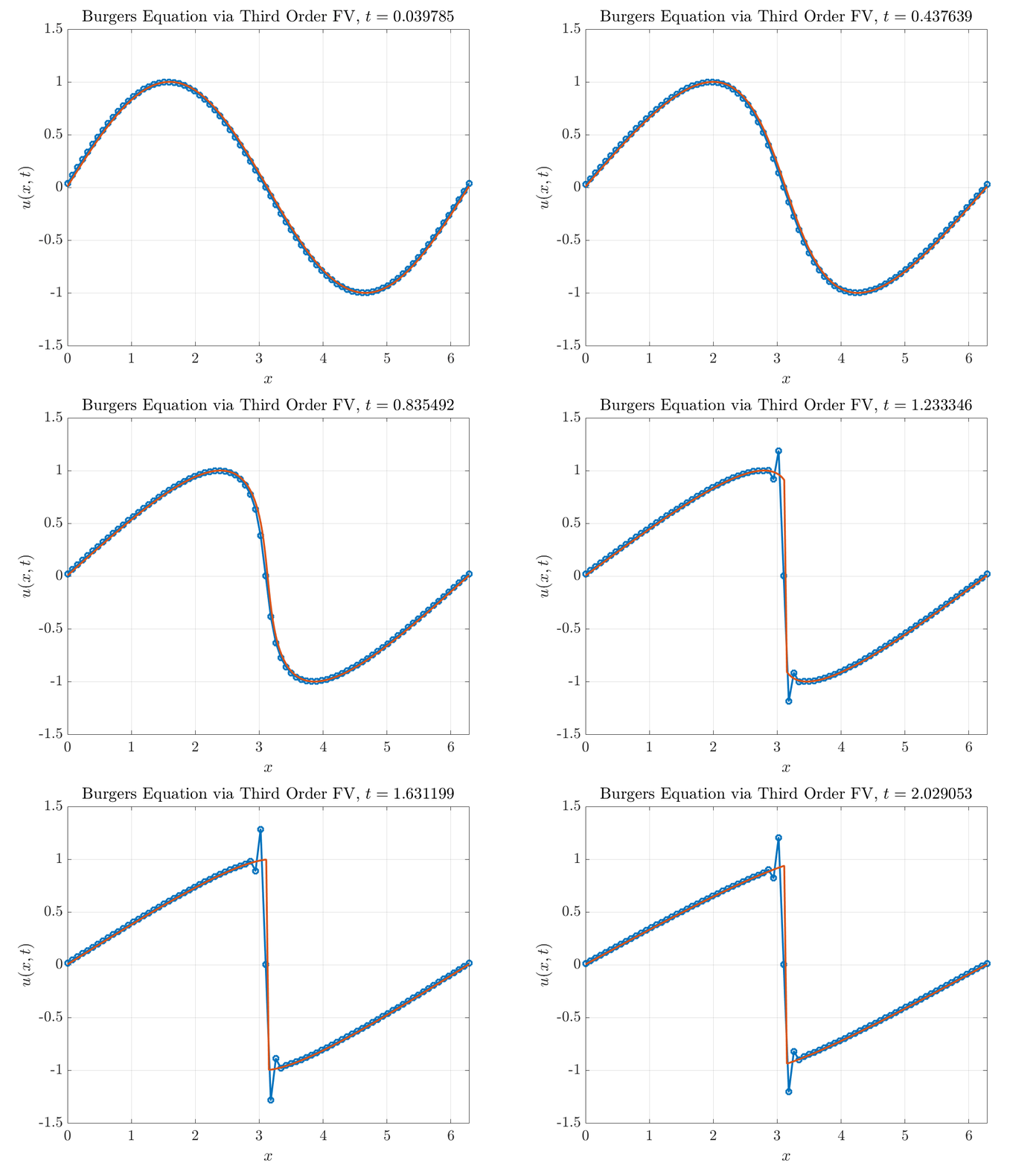
Yikes. On first glance, it appears our scheme performs reasonably well before the appearance of the shock but develops spurious oscillations after the shock. We can also compute the errors in the \(\ell^{1}\) norm:
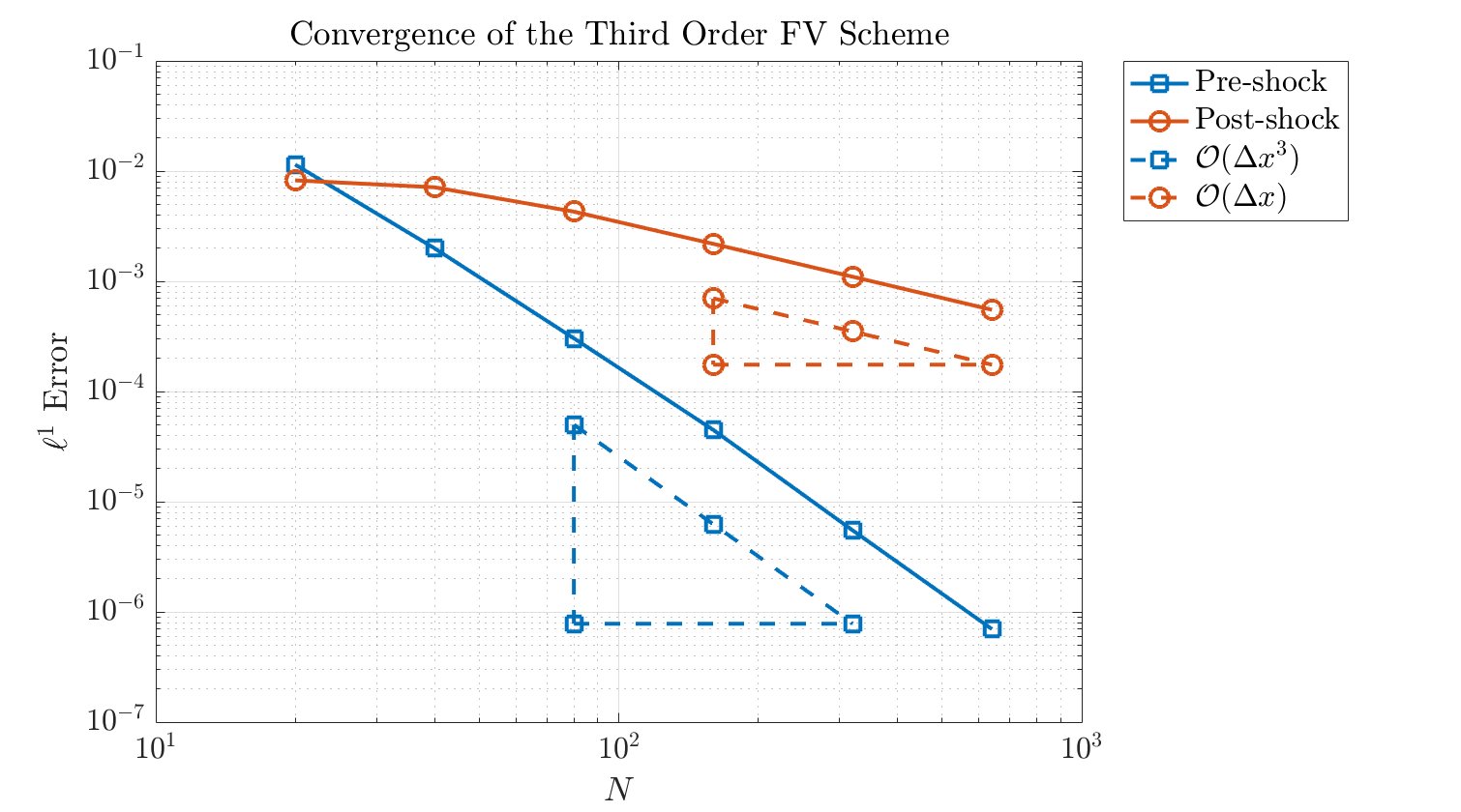
\[||\bar{u} - \bar{u}_{e}||_{\ell^{1}} = \frac{1}{N} \sum_{j=1}^{N} |\bar{u}_{j} - \bar{u}_{e,j}|.\]Figure 4 describes how the \(\ell^{1}\) error decreases as we increase the number of grid points. Before the appearance of the shock, our scheme displays third order accuracy as expected. But after the appearance of the shock, the accuracy is reduced to first order.
So, what on earth is going on here? The driving idea behind higher order schemes is that we hope to converge to the exact (entropy) solution faster than the original first order scheme. In the presence of shocks and discontinuities, though, it seems as if our third-order scheme hasn’t given us any benefits. Indeed, it actually introduces oscillations, which is arguably worse than the first order scheme which we recall was provably monotone and TVD.
2. Godunov’s Theorem
Our initial results are actually not altogether unexpected and are actually a result of Godunov’s Theorem.
Definition 3. A linear scheme is one that can be written in the form
\[\begin{align} \bar{u}_{j}^{n+1} = \sum_{\ell=-k}^{k} c_{\ell}(\lambda) \bar{u}_{j+\ell}^{n}, \;\;\;\lambda = \frac{\Delta t}{\Delta x}\notag \end{align}\]when applied to a linear conservation law.
It’s worth noting that all of the finite volume schemes we have considered thus far are linear schemes (a fact which can easily be verified with pen and paper).
Theorem 1. (Godunov) A linear scheme is monotone if and only if it is total variation diminishing (TVD). Moreover, linear TVD schemes are at most first-order accurate.
There’s quite a bit to digest here, but we’ll start with the first statement. Recall from last time that monotone schemes converge to the entropy solution and are also TVD. Godunov’s Theorem states that for linear schemes, the notion of being monotone is equivalent to being TVD. The second statement is much deeper: it tells us that if we want to construct a linear monotone scheme, then it must be first-order accurate. In particular, we posit that the third-order finite volume scheme is neither monotone nor TVD.
In fact, monotone schemes are at most first-order accurate regardless of whether the scheme is linear or not. This suggests that we simply can’t develop high order monotone schemes. However, having only a TVD scheme is still desirable as it essentially guarantees our scheme will not generate spurious oscillations. And yet, Godunov’s Theorem tells us that if we stick to linear schemes, we can’t develop high order TVD schemes either.
Nevertheless, it is still possible to enforce the TVD property on the third-order finite volume scheme. To do so, we employ a post-processing step known as slope limiting. This results in a nonlinear TVD scheme which is does not produce spurious oscillations.
3. Slope Limiting
I. Generalized MUSCL Limiter
The key observation is that when nonphysical oscillations appear in the numerical solution, the gradients of the cell averages between successive cells rapidly change sign. Slope limiting procedures identify where these sign changes occur and reduce the gradient to zero in these regions. The procedure is as follows.
- Given \(\{u_{j+1/ 2}^{\pm}\}\) and the cell averages \(\{\bar{u}_{j}\}\), define
- Compute the modified quantities \(\tilde{u}_{j}^{\text{mod}}\) and \(\tilde{\tilde{u}}_{j}^{\text{mod}}\) according to \(\begin{align} \tilde{u}_{j}^{\text{mod}} &= \text{minmod}\{\tilde{u}_{j}, \bar{u}_{j+1} - \bar{u}_{j}, \bar{u}_{j} - \bar{u}_{j-1}\}\\ \tilde{\tilde{u}}_{j}^{\text{mod}} &= \text{minmod}\{\tilde{\tilde{u}}_{j}, \bar{u}_{j+1} - \bar{u}_{j}, \bar{u}_{j} - \bar{u}_{j-1}\}, \end{align}\)
where the \(\text{minmod}\) function is defined as
\[\begin{equation} \text{minmod}(a_{1},\dots,a_{n}) = \begin{cases} s \cdot \min_{j} |a_{j}|, &s = \text{sgn}(a_{1}) = \dots = \text{sgn}(a_{n})\\ 0, &\text{else}. \end{cases}\notag \end{equation}\]- Compute the modified reconstructed values \(u_{j+1/ 2}^{\pm,\text{mod}}\) according to
The procedure outlined above is known as the generalized MUSCL (monotone upwind scheme for conservation laws) limiter. Note that the quantities \(\bar{u}_{j+1} - \bar{u}_{j}\) and \(\bar{u}_{j} - \bar{u}_{j-1}\) are crude approximations to the gradient over stencil \(\{I_{j}, I_{j+1}\}\) and \(\{I_{j-1}, I_{j}\}\). In the case of oscillations in our numerical solution, these two quantities will have opposite signs, in which case the \(\text{minmod}\) function returns $0$ and the modified quantities \(u_{j+1/ 2}^{\pm,\text{mod}}\) are set to the cell average. This is equivalent to the original first order finite volume scheme we studied last time! Hence, in the presence of shocks and discontinuities, we might expect the generalized MUSCL scheme to be first order accurate.
Now, let’s consider the case when the $\text{minmod}$ function returns the first argument. We carefully note that this situation occurs when \(\{\bar{u}_{j}\}\) is monotone over the stencils \(\{I_{j-1}, I_{j}, I_{j+1}\}\). Then we have \(u_{j+1/ 2}^{\pm,\text{mod}} = u_{j+1/ 2}^{\pm}\) and the high order finite volume scheme is unchanged. Thus, in smooth, monotone regions the generalized MUSCL limiter maintains original high order accuracy of the scheme.
Lastly, we must consider what happens near smooth extrema. For instance, \(u(x,0) = \sin{x}\) has smooth extrema at \(x=\pi/2\) (maximum) and \(x=3\pi/2\) (minimum). As consecutive gradients have opposite sign at local extrema, the $\text{minmod}$ function will return \(0\) and the scheme is again reduced to first order. Stanley Osher proved the following result:
Theorem 2. TVD schemes are at most first-order accurate near smooth extrema.
This seems like a problem since plenty of smooth solutions have smooth extrema. We’ll discuss shortly how to develop slope limiters which do not have this drawback, but first, it would be prudent to discuss to discuss the properties of the generalized MUSCL limiter. When paired with this limiter, the finite volume scheme is actually TVD. The proof is due to Ami Harten [2].
Lemma 1. (Harten) If a scheme can be written in the form
\[\begin{equation} \bar{u}_{j}^{n+1} = \bar{u}_{j}^{n} + C_{j+1/ 2}(\bar{u}_{j+1}^{n} - \bar{u}_{j}^{n}) - D_{j-1/ 2}(\bar{u}_{j}^{n} - \bar{u}_{j-1}^{n}) \end{equation}\]where \(C_{j+1/ 2}, D_{j+1/ 2} \geqslant 0\) and \(C_{j+1/ 2} + D_{j+1/ 2} \leqslant 1\), then the scheme is TVD.
Harten’s Lemma is the key to proving that the finite volume MUSCL scheme is TVD.
Proposition 1. The finite volume scheme with generalized MUSCL limiter is TVD.
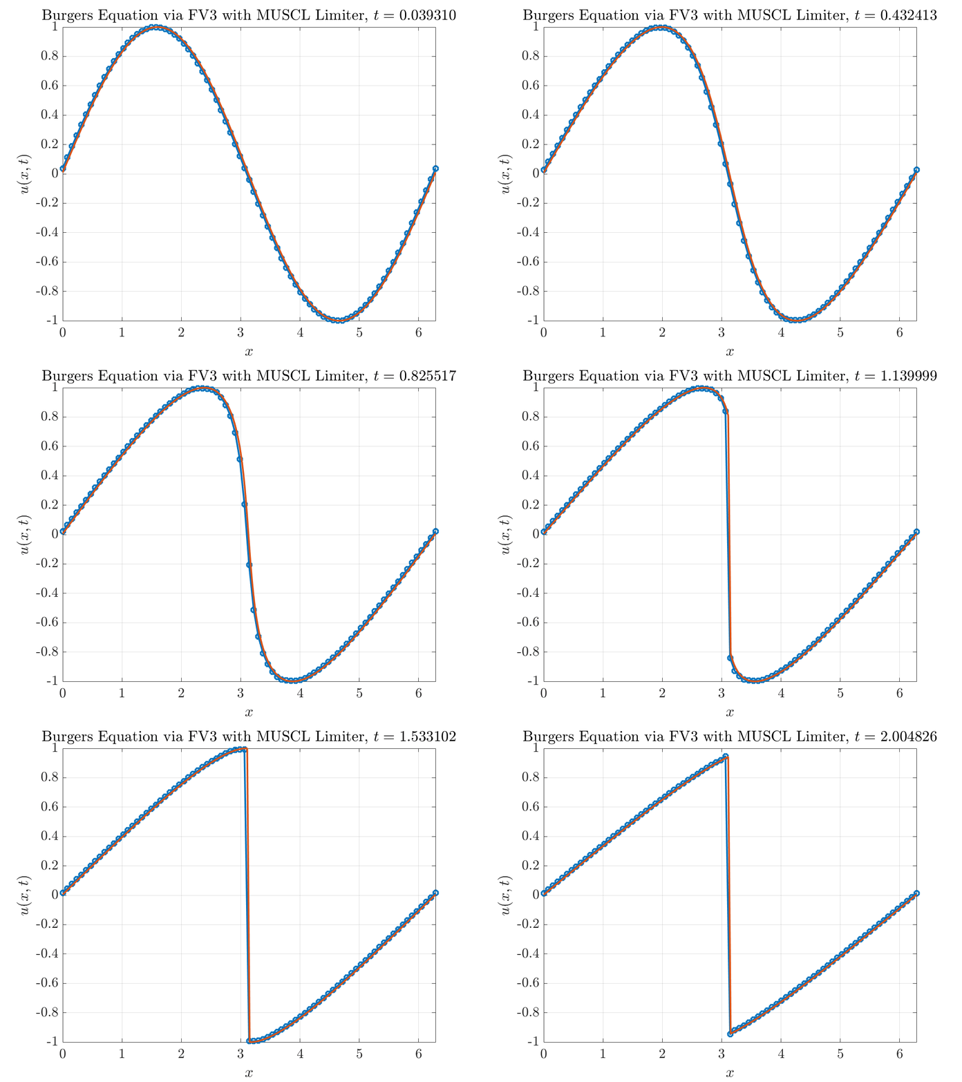
Without further ado, we present the results using the MUSCL limiter. The only change from the previous third-order code is to add the MUSCL limiter:
The \(\text{minmod}\) function is easily implemented as follows:
Figure 5 contains the results. Voila! At first glance, all appears to be well. The nonphysical oscillations have been removed entirely from our numerical solution.
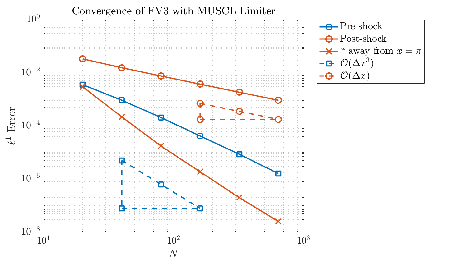
The next step is to verify that we are indeed getting the expected rates of convergence. There are three scenarios to consider: (i) the solution is smooth everywhere (we’ll consider the case when \(T=0.3\)) (ii) the solution develops a shock and we compute the \(\ell^{1}\) error over the entire computational grid (we’ll consider the case \(T=1.5\) here) (iii) the solution develops a shock and we compute the \(\ell^{1}\) error excluding a small region around the shock.
In the first scenario, we expect a reduced rate of convergence due to the presence of smooth extrema in the solution. In the second scenario, the order of convergence should be reduced to first order. Finally, in the third scenario, the solution is actually piecewise monotone and so we might expect to maintain the original third order accuracy if compute errors away from the shock.
Indeed, Figure 6 shows these three scenarios exactly. Before the shock, the overall order of accuracy is somewhere between 2 and 3; at the two extrema, the order is reduced to 1 but everywhere else, it is close to 3, leading to a suboptimal order of accuracy. After the shock, the order of accuracy is 1 overall, but when considering only cells at a distance 0.5 away from the shock at \(x=\pi\), the order of accuracy is 3.
This isn’t such a bad place to be, then. Near shocks, the mathematical theory tells us that we can never do better than first order accuracy, but we’ve managed to construct a scheme which is TVD and capable of giving higher order accuracy everywhere the solution is smooth. In the end, this is all we can really ask for. In the remaining posts, we will consider the different types of high order schemes which can be used to numerically solve nonlinear conservation laws.
II. Total-Variation Bounded (TVB) Limiter
But first, we consider how to remedy the issue of suboptimal convergence near smooth extrema. Recall that the issue here is that consecutive gradients have different signs and the \(\text{minmod}\) function return zero. In fact, recall that Theorem 2 tells us we can have at most first order accuracy near smooth extrema. If we relax the TVD constraint even further, it is possible to obtain uniformly high-order accurate schemes near smooth extrema.
Definition 4. If \(TV(\bar{u}^{n}) \leqslant B\) for some fixed \(B>0\) depending only on \(TV(\bar{u}^{0})\) and \(n\) and \(\Delta t\) such that \(n\Delta t < T\), then the scheme is said to be total variation bounded (TVB) in \(0 \leqslant t \leqslant T\).
It is clear that all TVD schemes are TVB. For TVB schemes, one can show that there exists a subsequence in \(L^{1}_{\text{loc}}\) that converges to a weak solution of the conservation law.
In order to turn the generalized MUSCL limiter into a scheme that is TVB, we need only make a small adjustment. Namely, we define
\[\begin{align} \tilde{u}_{j}^{\text{mod}} &= \overline{\text{minmod}}\{\tilde{u}_{j}, \bar{u}_{j+1} - \bar{u}_{j}, \bar{u}_{j} - \bar{u}_{j-1}\}\notag\\ \tilde{\tilde{u}}_{j}^{\text{mod}} &= \overline{\text{minmod}}\{\tilde{\tilde{u}}_{j}, \bar{u}_{j+1} - \bar{u}_{j}, \bar{u}_{j} - \bar{u}_{j-1}\},\notag \end{align}\]where the modified minmod function \(\overline{\text{minmod}}\) is defined by
\[\begin{equation} \overline{\text{minmod}}(a_{1}, \dots, a_{n}) = \begin{cases} a_{1}, &|a_{1}| \leqslant M\Delta x^{2}\\ \text{minmod}(a_{1}, \dots, a_{n}) &\text{else}. \end{cases}\notag \end{equation}\]Here, \(M>0\) is a parameter to be chosen by us. Essentially, the TVB limiter first checks whether \(u_{j+1/ 2}^{-}\) is sufficiently close to \(\bar{u}_{j}\). If so, then the modified $\text{minmod}$ function returns the first argument even if consecutive gradients have different signs, thus ensuring that the scheme retains high-order accuracy around smooth extrema [4]. The implementation is quite straightforward:
We won’t show plots of the numerical solution here as they wouldn’t be discernible from the plots of the MUSCL limiter to the naked eye. Instead, Figure 7 shows the convergence rates for the TVB limiter. We note that before the shock forms, the order of accuracy is now 3 as expected, even in the presence of smooth extrema.

4. Key Takeaways
To summarize, we implemented a third order finite volume scheme for a one-dimensional scalar conservation law. Without any modifications, this scheme was not TVD and introduced new extrema in our numerical solution that were not seen in the first order finite volume scheme. We touched on Godunov’s Theorem, which describes the fundamental limits of accuracy of linear monotone schemes.
We were able to develop a TVD slope limiter to remove the spurious oscillations in our high order numerical solution but noted that the limiter degraded the order of accuracy of our scheme near smooth extrema. In fact, we learned that all TVD schemes are at most first order near smooth extrema. To develop a truly high order scheme in the presence of smooth extrema, we turned to the TVB limiter.
It is worth emphasizing once more than when we talk about “high order” schemes for nonlinear conservation laws, we generally mean that the scheme maintains high order accuracy in smooth regions, is first order accurate in the vicinity of shocks and discontinuities, and is total variation diminishing (does not introduce any new extrema/spurious oscillations). Next time, we will cover essentially non-oscillatory finite volume schemes which essentially remove spurious oscillations by performing the polynomial reconstruction step in a clever way rather than post-processing the reconstruction as with the slope limiters we have seen in this post.
References
[1] Gottlieb, Sigal, and Chi-Wang Shu. “Total variation diminishing Runge-Kutta schemes.” Mathematics of computation of the American Mathematical Society 67.221 (1998): 73-85.
[2] Harten, Ami. “High resolution schemes for hyperbolic conservation laws.” Journal of computational physics 49.3 (1983): 357-393.
[3] Johnson, B. Cockburn C., and C-W. Shu E. Tadmor. “Advanced numerical approximation of nonlinear hyperbolic equations.” (1997).
[4] Shu, Chi-Wang. “TVB uniformly high-order schemes for conservation laws.” Mathematics of Computation 49.179 (1987): 105-121.
Codes & Resources
- NumCL repository on GitHub
- Figures 1 and 2 were created using Mathcha, an online math editor with a convenient GUI that even allows you to export figures to TikZ.